Most cities played in 24 hours

The problem
Laying out
Solving the problem
Results

How many cities can a band play in within only 24 hours?

This was inspired by the Crywank tour in which they played 16 shows in the UK, in only 24 hours.

Thinking about it, maybe there would have been a way to compute the maximum amount of cities playable at using graph theory…

Of course you can skip to the results right away.

The problem

Suppose we have a set \(S\) of points representing cities. Let \(G = (S, A)\) an oriented graph. Let every edge \((a, b) \in A\) have a weight being the travel distance (in seconds) between city \(a\) and city \(b\).

We are going to assume that the band travels in a car that can go at \(50km/h\) on average. This way, we can easily calculate the travel distance between two cities by dividing their Euclidean distance (in km) by the speed of the car.

Let’s assume every gig takes no more than 20 minutes. To that, let’s add 5 minutes of setting-up and 5 minutes of getting everything back in the car. When it’s over, the band immediately starts to travel to the next city.

We want to find a path of \(n\) vertices in \(G\) that verifies the following conditions:

the total weight is less than \((24\times60\times60) + n \times (30\times60)\), so \(86400 + n \times 1200\) (time to travel + time to play the gigs)
it has the maximum possible amount of vertices

It resembles the traveling salesman problem and the longest path problem, but after some research these turned out to be very different…

Laying out

Fortunately, a course held this semester focused on graph algorithmics. And by chance, a dataset of 6 to 112 points representing the cities of France was handed out during a practical exercise (I alternate between them over the post to show different examples).

However, we still have to input the edges ourselves.

First of all, the graph clearly doesn’t need to be complete: it is not useful to connect two cities on the far ends as they will have a huge weight.

I chose to use a Delaunay triangulation to connect the cities. I used Numpy and Scipy to triangulate the points.

Here’s the entire map we’re going to use (ignore the fact that the roads to Ajaccio and Bastia are technically underwater):

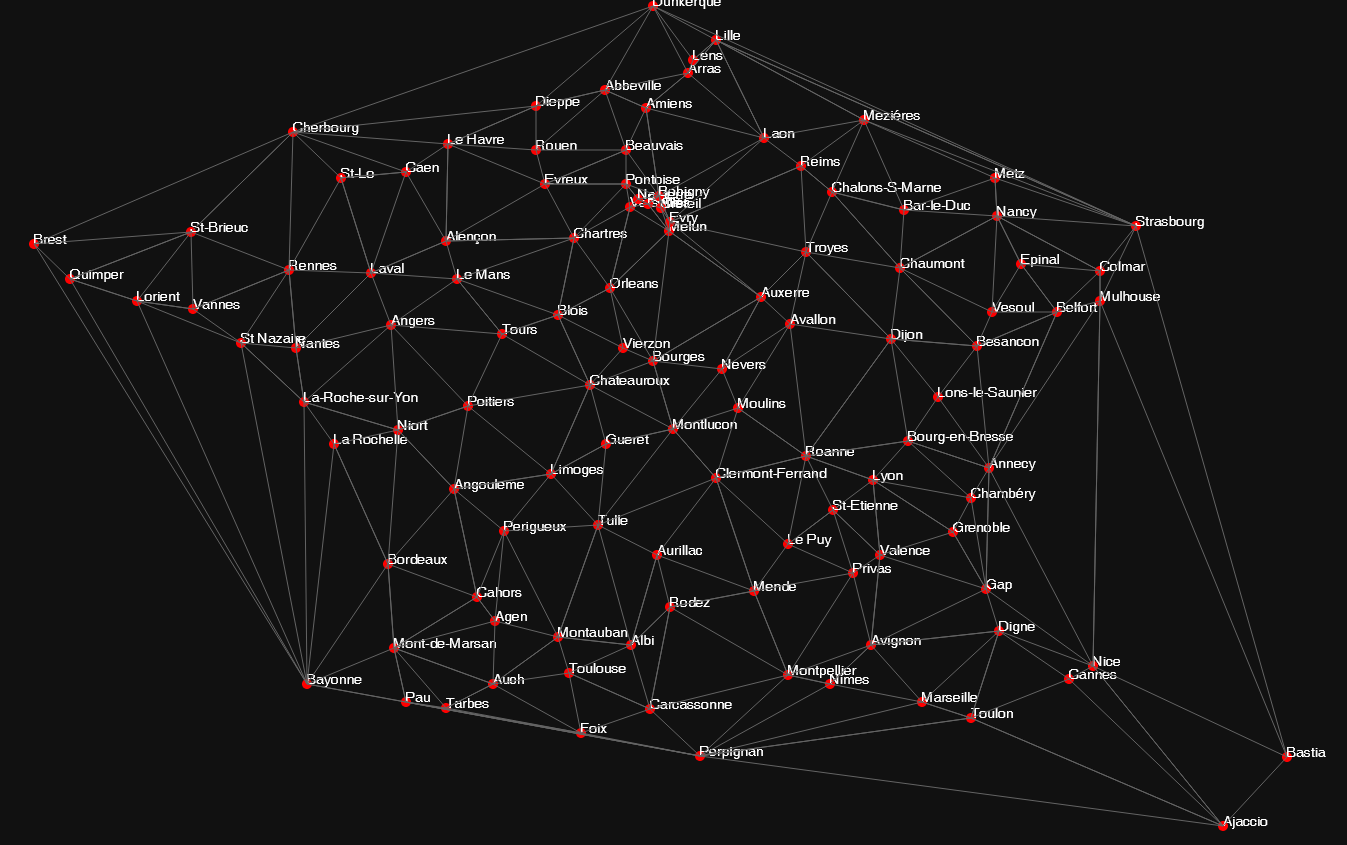
Now, let’s compute the weights. Fortunately, the dataset had realistic coordinates so the Euclidean distances matched when I computed them. Dividing the distance by a carSpeed variable gives us the travel time from one city to another.

Solving the problem

After thinking and researching multiple methods (including brute-forcing everything, using Hamiltonian cycles and using minimum spanning trees), I came up with this algorithm:

Initialization

pick a start vertex as a starting point for the path
initialize total_time to 0
initialize visited to an empty list (the list of visited cities)
let ends = (a, b) a couple representing the two vertices on the two ends of the path: initialize it as (start, start)

While total_time < maximum_total_time

check if adding 30 minutes to total_time still satisfies the condition
- if so, add the time. If not, break the loop
compare the weights of all the edges that come from ends.a or ends.b, except those leading to a vertex in visited. Then get the edge of form (from, next) with the minimal weight
add from to visited
check if adding the travel time from from to next to total_time still satisfies the condition
- if so, add the time. If not, break the loop
if from == ends.a, then ends.a = from. Same for ends.b

In the end, the number of cities visited is the length of the visited list, and total_time is the play time plus the travel time. Travel time (time spent moving between cities) and then play time (time in cities) are easily computable.

It took less than 0.01 second to execute in Python with the 112 cities dataset. Here’s an output with a random starting point:

112 cities dataset: 21 cities played (random starting point)

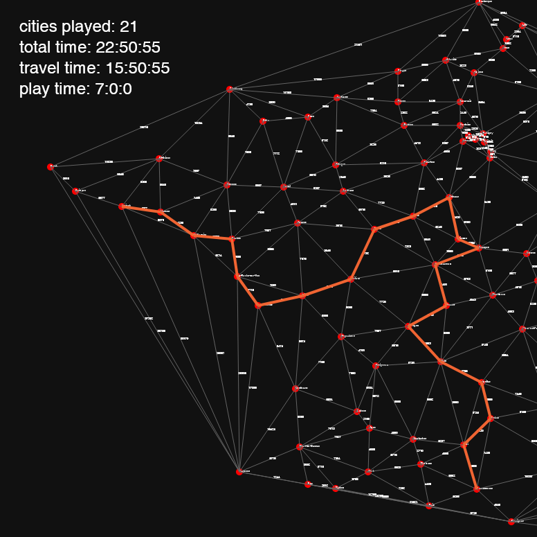
Turns out there already is a way to beat the 16 cities record.

Picking a starting point

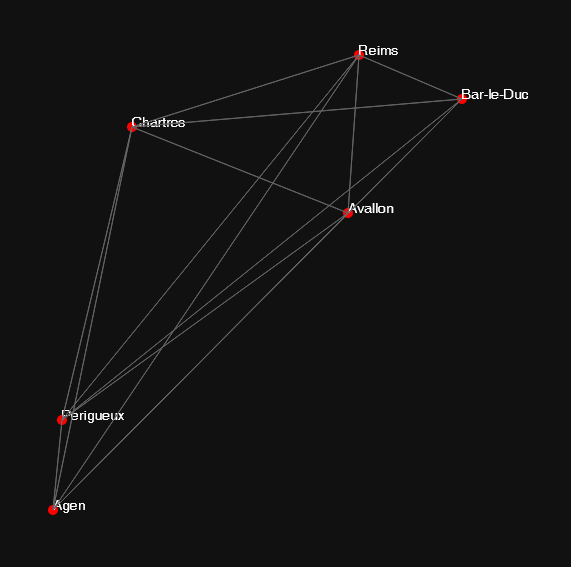
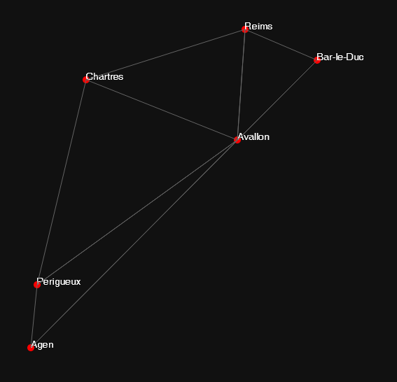
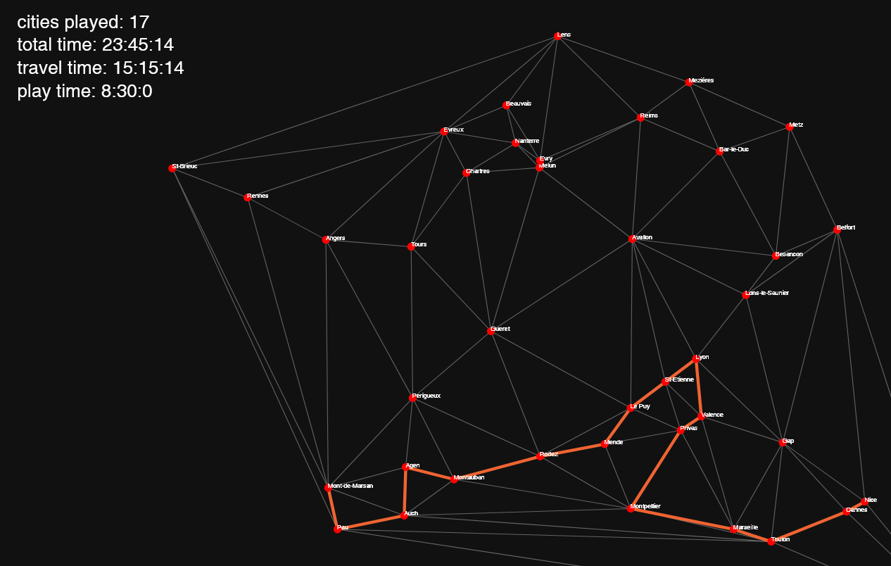
The starting point choice is crucial as two different points can produce different paths:

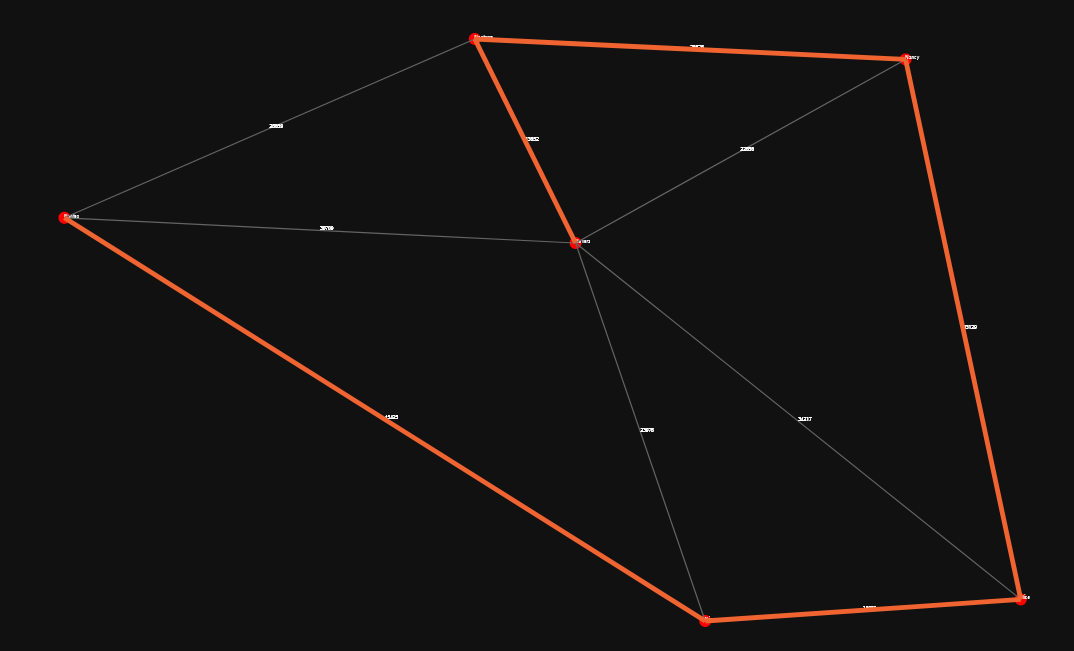
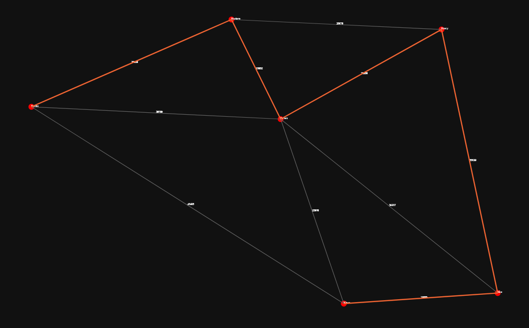
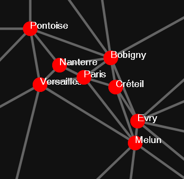
As you may have seen in the 112 cities dataset, there is quite a huge cluster of cities near Paris. Therefore, these vertices are interconnected with edges having very small weights. Which would make a great starting point, as multiple cities could quickly be covered.

I used this idea to make a first findLowestSumVertex() function that calculates the sum of the weights of the edges for every vertex, and then returns the vertex with the lowest sum. This function should return a point that is very close from other points, hence its lowest sum of edge weights.

Now here’s an example of why that couldn’t work… If we have a cluster \(A\) of 5 very close cities, and another cluster \(B\) of 10 less close cities, the two clusters being very very far from each other (let’s say a travel distance of 24 hours). findLowestSumVertex() will clearly return a point in cluster \(A\), which means that it will then have to travel 24 hours until it reaches cluster \(B\). This will not find the path with the most cities, as it will only stay in the 5 cities cluster and never reach the 10 cities cluster.

The second and final method is to run the algorithm n times and make it return the number of visited cities. By testing every vertex as a starting point, it ensures that there is no omitted path. Then, we could get the vertex that maximizes the output of the algorithm when used as a starting point, and use this vertex as a starting point.

Results

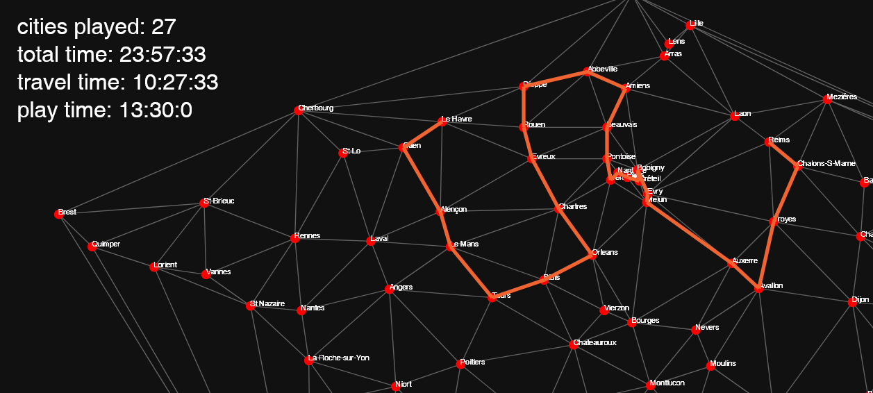
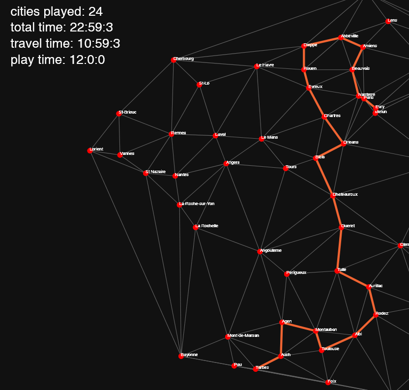
When running the full algorithm on the 112 cities dataset, we get this path of 27 cities:

Here are other results with less cities. Of course, the dataset can be modified to only include big cities, to make the tour more interesting.

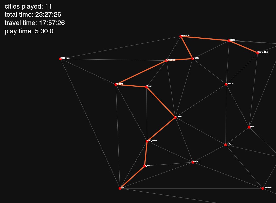
There is a huge difference between the play time and the travel time on this 20 cities dataset. But since we only care about the record, that’s fine.

There is no formal proof that these are optimal paths, but they seem to work alright.

As a conclusion, the record of the most cities played in 24 hours could be beaten in France! If you don’t sleep, that is.